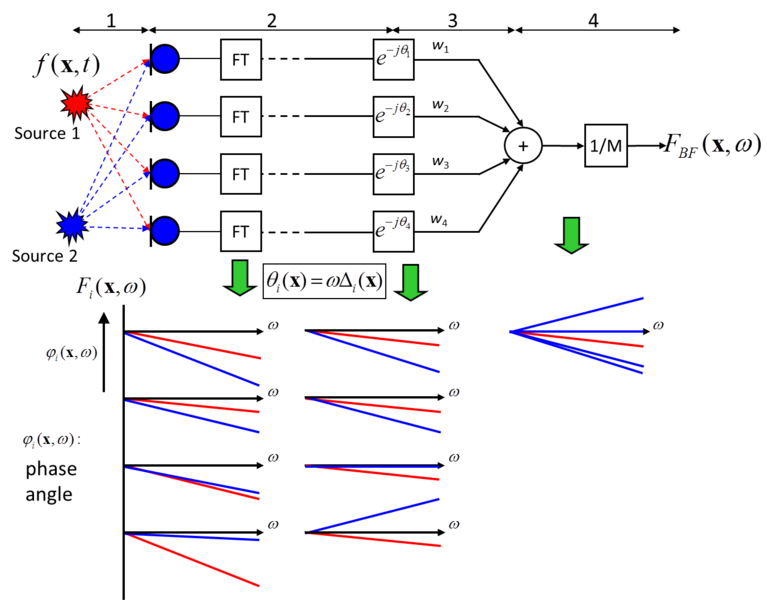
The delay summation beamformer in the frequency domain is based on principles similar to those in the time domain. The block diagram in the figure illustrates the situation of two point sources located in the measurement plane in front of the microphone array.
The sound from each sound source propagates along different paths to each microphone. This will result in the delay and phase of the measurement signal, both of which are proportional to the travel distance. The delay can be determined based on the known distance and sound velocity between the microphone array and the measurement plane.
After performing Fourier transform on each microphone signal, the spectrum can be used as amplitude and phase. Now, the phase of each individual microphone signal can be corrected based on a specific delay. It is multiplied by a complex phase term without affecting the amplitude. The figure provides an example of this process. Here, the phase adjustment of the signal section is performed for target source 1. Therefore, the signal of source 2 is partially out of phase. It is important to note that a constant time delay can lead to frequency dependent phase correction terms.
Add the complex spectra obtained. During this process, the signal portion of source 1 accumulates constructively, while the signal portion of source 2 decreases.
Finally, the sum signal is normalized by the number of microphone channels. RMS values and maximum values can be calculated from the sum spectrum and visualized in the acoustic map. In order to hear the sound signal at the focal point, an inverse Fourier transform can be performed to generate a local time signal (f_ {BF} (x, t) ) at the focal point. F B F (X,) is at the focal point.